Factor Analysis is used in experiments where n correlated variables are measured, and the researcher wants to extract a set of m≤n latent variables, that represent the variability of the original data as closely as possible.
These new variables are the so-called factors (nothing to do with the concept of a 'factor' variable in R), which are mutually independent, linear transformations of the original variables. The linear relation between both sets of variables is represented by a matrix of n�m coefficients or loadings. For each possible combination of the original variables, this matrix determines a projection in the sub-space spanned by the factors, and the objective of the analysis is to achieve minimal differences between the original observations and their projections in that sub-space.
Any scaling of each factor by a constant would represent an equivalent solution to the problem. In order to standardize the results, the loadings matrix contains the Pearson correlations between factors and variables. This is an univocal scaling, where loadings are always in the range [-1, 1], and their sums of squares along each factor is proportional to the amount of variance explained by that factor.
Note: This dialog uses the functions fa and principal of package psych, not factanal from the standard stats package. Notice that the results of principal are those of a factor analysis using the extraction method of principal components, not the results of a principal components analysis (like princomp or prcomp). See more information on these methods in the following links:
The main dialog is used to select the original variables from a data frame of the workspace, and the number of factors that will be defined. This is an arbitrary number chosen by the researcher, although parts of the results in a first trial may be used to redefine the model with a different number of factors.
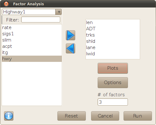
There also are two buttons for plotting some results and setting some options of the analysis, as explained in the following sections.
This sub-dialog is used for setting the options of the analysis:
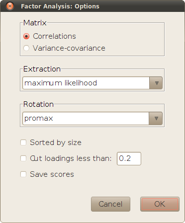
factanal as well (but not the default of fa).
X.1 (where X stands for the name of the original data frame), that contains the n original variables selected for the analysis, plus the m scores.
This sub-dialog contains a list of check boxes for representing different plots:
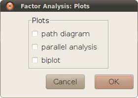
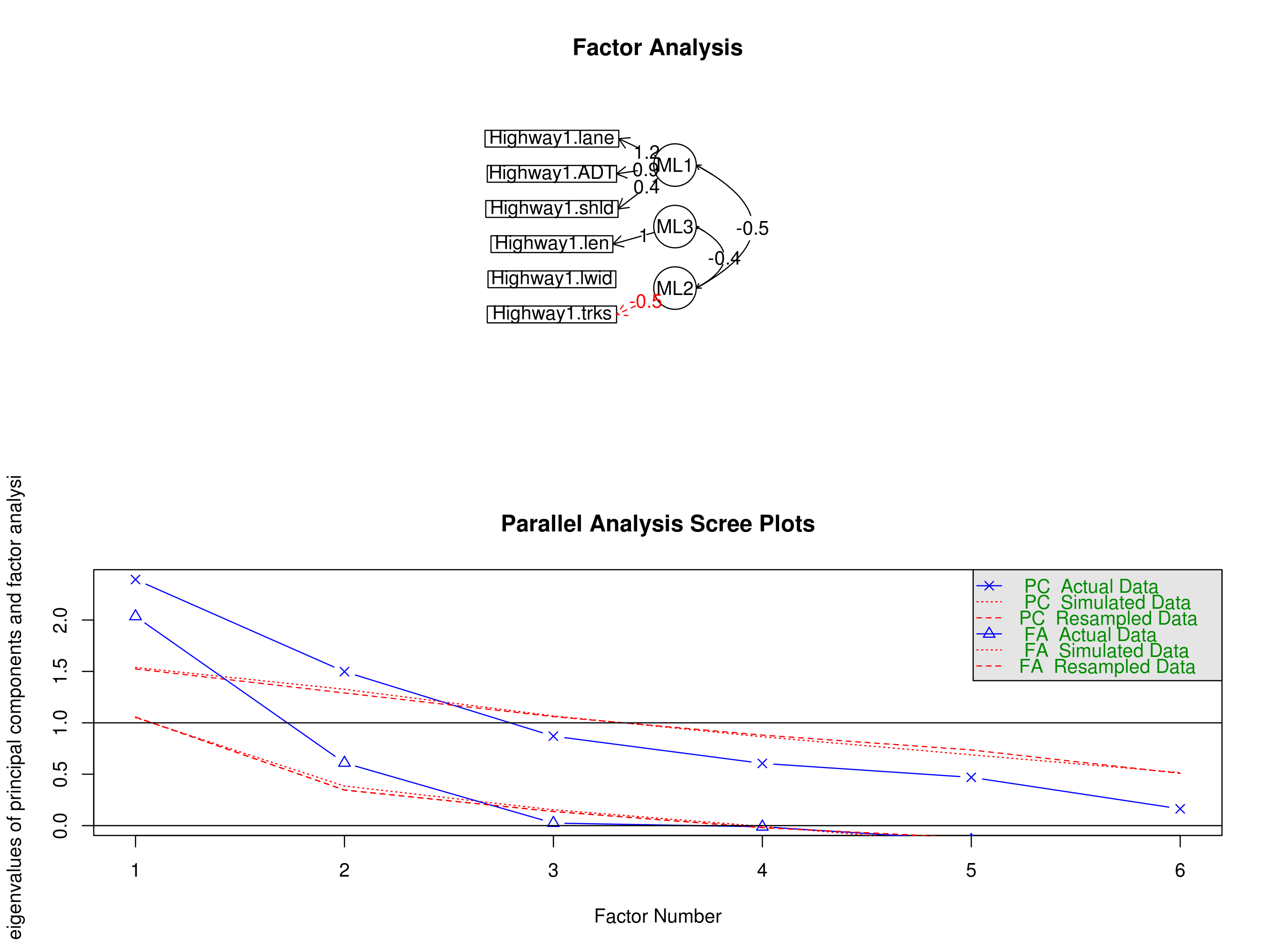
A visual representation of the correlations between original variables and factors: the former are drawn in rectangles, and the latter in circles. The variables and factors that have a correlation greater than 0.3 are graphically connected between them (this is the same information conveyed by the loadings matrix if the values are cut below 0.3). The correlations between different factors are drawn as well.
When there is no special reason for deciding the number of latent factors, researchers often take a decision based on the amount of variance explained by the first factors (ordered by explanatory power), and the gain obtained for additional factors, as seen in 'scree plots'. The parallel diagram prints such plots for the observed data and artificial, random uncorrelated data used as baseline. The crossing between these scree plots may be used for 'suggesting' number of factors, as the maximum number that explains an amount of variance of the actual data proportionally greater than for the artificial data (before both scree plots cross). The plots are printed for two representative methods of factor extraction (principal components and principal axis factoring), regardless of the method actually set in Options (see below). If the path diagram is also selected, the parallel analysis is shown below in the same figure.
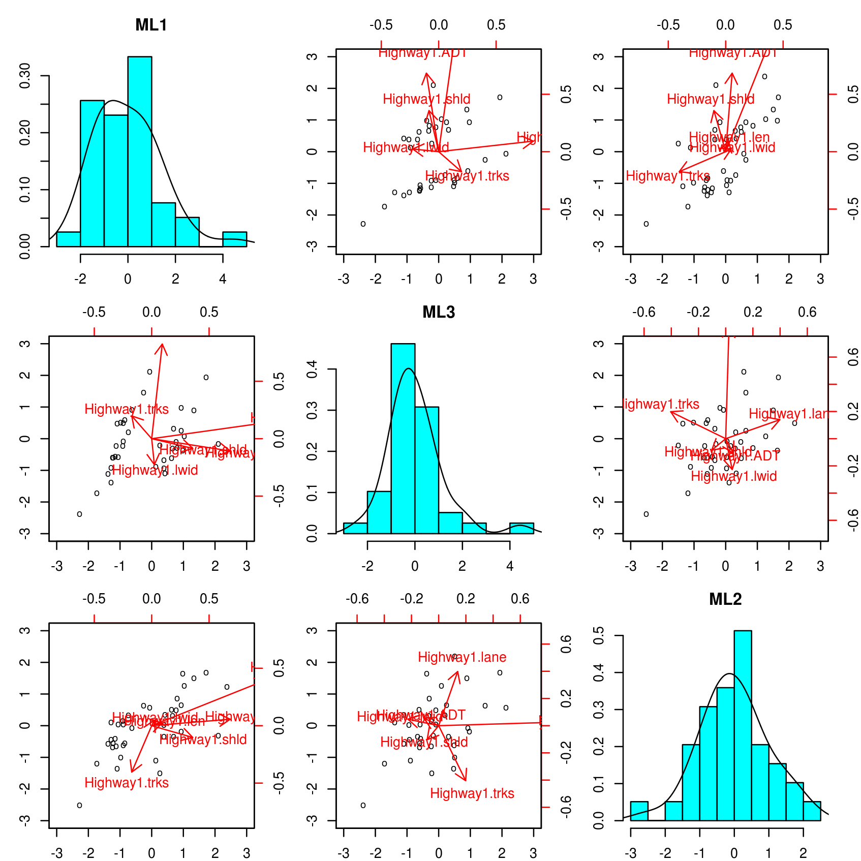
This plot represents a matrix of scatterplots and histograms, with the projections of the observed data in different planes of the sub-space spanned by the extracted factors. This may be used to see how the observations are distributed along the scale of the different factors. The superimposed arrows are projections of the original variables in those planes, defined from the vectors (columns) of the loadings matrix; the longer and more parallel to the horizontal or vertical axis, the stronger will be the relation between the represented variable and the factor corresponding to that axis. This essentially is what the path diagram represents as well, although the information of the biplots is more comprehensive (and also more difficult to grasp if the number of factors is greater than two or three).
