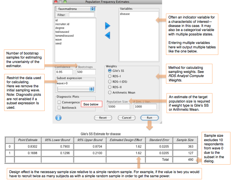
This dialog computes a point estimate and confidence interval of population frequency (prevalence), for one or more categorical variables. The input and output are shown below. The default method is Gile's SS estimator, where the confidence interval is computed using Gile's bootstrap method. This is a computationally-intensive procedure and can take a minute or longer to complete.
Convergence plots help to determine whether the final RDS estimate is biased by the initial convenience sample of seeds. If the estimates shown in the plots do not level off as the sample size increases then the current estimate is probably biased by the choice of seeds. It is recommended to create a convergence plot of all traits of interest during the research process and extend sampling if the estimate has not stabilized (Gile, Johnston, Salganik 2012).
The convergence plots below show a data set that has converged (left, using fauxmadrona sample data) and one that has not (right).
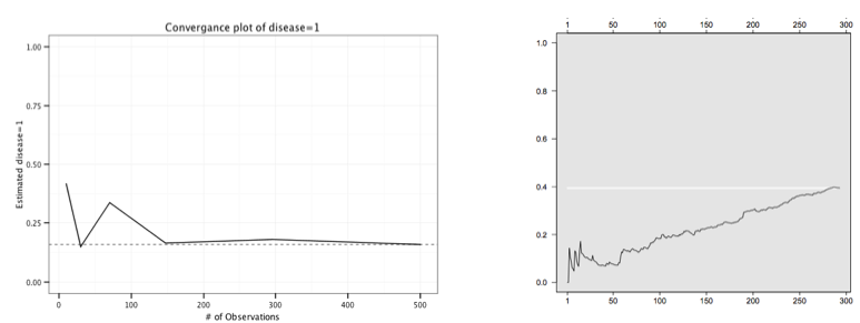
Note that although the plot on the left shows convergence, there is a chance that additional data would not follow this trend. The recruitment tree could be stuck in a sub-population of the population of interest. This is discussed further below.
Bottleneck plots are used to asses whether the population of interest contains distinct sub-communities that could bias the RDS estimate. If the sub-communities tend to recruit from within (i.e. exhibit homophily) then the choice of seeds may generate a biased sample. If the sub-communities are different with respect to the population characteristic of interest then the RDS prevalence estimate may also be biased.
An example of this scenario is described in "Diagnostics for Respondent-driven Sampling" (Gile, Johnston, Salganik 2012):
"Imagine a city with street-based sex workers and brothel-based sex workers where there are many social connections within these groups, but few connections between these groups. Further, imagine that brothel-based sex workers use condoms regularly, whereas street-based sex workers do not. This situation will be problematic for RDS because the network "bottleneck" between the two groups will prevent the sample from exploring the entire population and could lead to inaccurate estimates about both sex worker type (i.e., brothel-based vs. street-based) and condom usage."
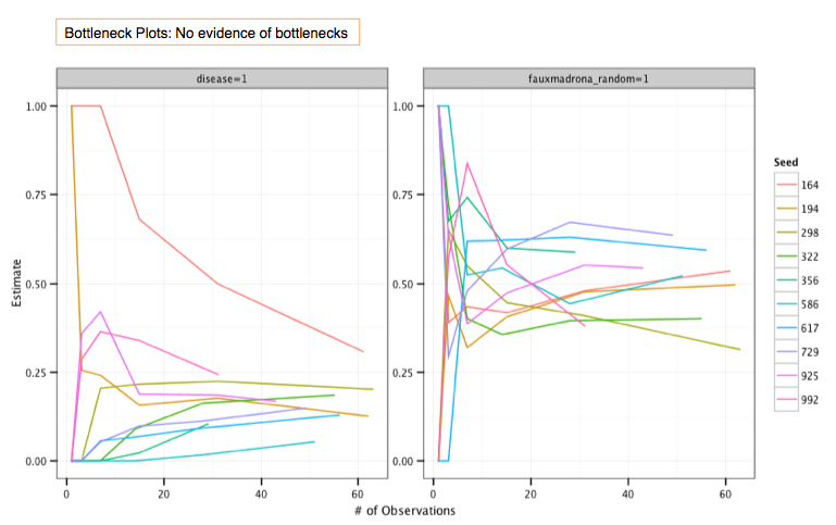
Each line of a bottleneck plots tracks an estimate of a characteristic of an interest based on one of the seeds. If the estimates converge as the samples from each seed (their trees) grow, then there is no indication of a bottleneck along this characteristic.
Below are two bottleneck plots prepared from the fauxmadrona data set. (To load fauxmadrona, select "Example: fauxmadrona" from the Packages & Data menu). Both track the samples originating from each of the 10 seeds, as labeled by ID in the legend at right. (Note that the lines for each seed end at different places, reflecting the different sizes of the trees that originate from each seed.) The plot on the left tracks the estimate of the prevalence of disease in the population. While the estimates start at a range of values, they all converge toward about 20%, showing no evidence of divided sub-communities of infected and uninfected. Similarly, the plot at right tracks the samples along a completely randomized 0/1 indicator variable for the population. As expected, the prevalence estimates of this indicator converge toward .5, with some variation around that estimate.
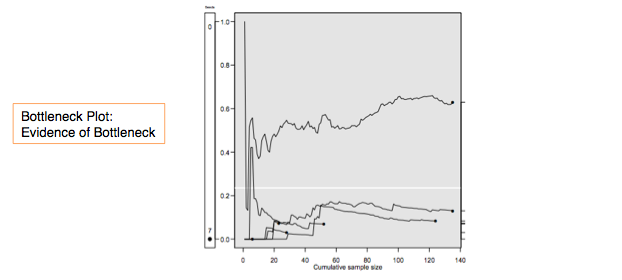
In comparison, a plot with evidence of bottlenecks (created in R) is shown below. The estimates stabilize at different places depending on where the seeds originate.
 Deducer: A GUI for R