Description

The generalized linear model (GLM) is a flexible generalization of the linear and logistic regression models. It can be used to model outcomes with a variety of different distributions, and different relationships to their predictors.

A general mathematical formulation can be found here, and a treatment in R can be found here.

Variable Selection

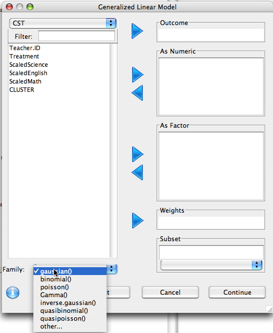
This dialog is used to define what variables are of interest, and how they should be treated.

Outcome Variable: The dependent variable should be put in this list
As Numeric: Independent variables that should be treated as covariates should be put in this list. Note that if a factor is put in this list it is converted to a numeric variable using the as.numeric function, so make sure that the order of the factor levels is correct.
As Factor: Independent variables that are categorical in nature should be put here (e.g. race or eye color).
Weights: This advanced option allows for sampling weights to be applied to the regression model.
Subset: As with many other dialogs in Deducer, you can specify that the analysis is only to be done within a subset of the whole data set.
Family: The Family of model to be fit

Model Builder

R has a rich syntax for expressing model formulae. The model builder dialog assists in the specification of the terms of a model.

Outcomes

Only one outcome is allowed. It can be edited by double clicking on it.

Model

Select one or more variables from the Variable list, the click on one of the center buttons to add a term to the model.

2-way Add all two way and lower interactions between the selected variables.
3-way Add all three way and lower interactions between the selected variables.
+ Add Main effects for all selected variables.
: Add the interaction between the selected variables to the model.
* Add the interaction between the selected terms, as well as any lower order interactions between them.
- Remove a term from the model.
in Add a nested term to the model
poly Add orthogonal polynomial terms to the model. A dialog will prompt for the order of the polynomial. If the order is two, this indicates a linear and quadratic term. If it is three it will also have a cubic term. Polynomials can be used when there is non-linearity detected between the outcome and a predictor.

Additionally, terms can be hand edited by double clicking on them.

Model Explorer

After the model has been built, its features can be explored. The preview panel displays a preview of what will be displayed in the console when the model is run. In the upper left hand portion of the dialog there are icons representing the assumptions that are being made by the model.

The following analysis options and dialogs are available

Additionally, several plots can be accessed through the upper tabs to help diagnose the fit of the model.

Diagnostics

The diagnostics panel contains 4 plots evaluating outliers, influence, and equality of variance.

The first two plots describe the distribution of the residuals. Ideally these should be roughly normal.

Cook's distance Outliers can unduly influence the results of the model. This plot shows the row names for observations with moderate or high cook's distance. If the Cook's value is greater than 1, the observation should be examined.

Residuals vs. Leverage A plot to examine influence and outliers.

Term plots (aka Component residual or partial residual plots)

If the model contains no interactions, component residual plots are given. These are used to assess the linearity of the relationship between predictor variables and the outcome.

For numeric variables, a scatterplot is produced. If the trend line of this plot shows departure from linearity, consider either transforming the variable, or adding polynomial terms to it.
For factors, box-plots are given. If a factor has more than two levels, is ordinal, and appears to be linearly increaseing or decreasing, consider going back and adding it to the model as a numeric variable.

GeneralizedLinearModel {Main}