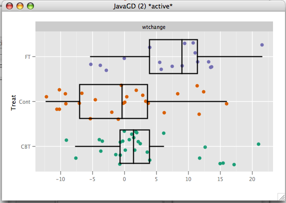
Data contains pre and post treatment weights for 72 young women who underwent treatment for anorexia.
enter the following into the console:
data(anorexia)
anorexia$wtchange <-anorexia$Postwt - anorexia$Prewt
Variables:
We are interested in change in weight, so wtchange is moved to the outcome list. Our groups are defined by the treatment variable Treat. We will also construct a plot.


k.sample.test(formula=d(wtchange) ~ Treat,
		data=anorexia,
	test=oneway.test)
oneway.plot(formula=d(wtchange)~Treat,data=anorexia,
	alpha=1.0)
>k.sample.test(formula=d(wtchange) ~ Treat,
+ data=anorexia,
+ test=oneway.test)
                           One-way analysis of means (not assuming equal variances)
                F (num df,denom df)     p-value
wtchange 5.355442        (2,41.136) 0.008568491
> oneway.plot(formula=d(wtchange)~Treat,data=anorexia,
+ alpha=1.0)

From the plot we see that there are no outliers, and the distributions are not very skewed, thus it is appropriate to use an Anova. The Anova analysis found that the means of the three groups were significantly different (p=.00857). From the plot we see that both the girls put in the CBT group and the FT group gained weight, whereas the Cont group actually lost weight. Those in the FT group experienced the most weight gain. A Two Sample Test could be used to do the pairwise comparisons between the groups.